ML

Computing the product of Gaussian distributions

November 26, 2022

Suppose you have \(K\) multivariate Gaussian distributions, each of dimensionality \(N\). It turns out that the product of these distributions, after normalization, is also multivariate Gaussian. What is the algorithmic complexity to compute this product?

Let's first assume that each \(k\) of the \( K\) Gaussian distributions is parameterized by mean \(\mu_k\) and covariance \(\Sigma_k\). The product is proportional to a Gaussian with mean \(\mu\) and covariance \(\Sigma\), where

\[\begin{aligned} \mu =& \Big(\sum^K_{k=1}\Sigma_k^{-1}\Big)^{-1} \Big(\sum^K_{k=1} \Sigma_k^{-1} \mu_k\Big), \\ \Sigma =& \Big(\sum^K_{k=1}\Sigma_k^{-1}\Big)^{-1}. \end{aligned} \]

Assuming we have memory to store and reuse all intermediate results, we will need to perform \(K+1\) matrix inversions and to solve \(K+1\) linear systems. Thus, the runtime complexity is \(O(KN^3 + KN^2)=O(KN^3)\).

Now, let's instead assume that each \(k\) of the \( K\) Gaussian distributions is parameterized by mean \(\mu_k\) and precision (i.e. inverse covariance) \(\Lambda_k\). The product is proportional to a Gaussian with mean \(\mu\) and precision \(\Lambda,\) where

\[\begin{aligned} \mu =& \Big(\sum^K_{k=1}\Lambda_k\Big)^{-1} \Big(\sum^K_{k=1} \Lambda_k \mu_k\Big), \\ \Lambda =& \Big(\sum^K_{k=1}\Lambda_k\Big). \end{aligned} \]

Here, we only need to perform \(K\) matrix-vector products and solve \(1\) linear system. So the runtime complexity is \(O(KN^2)\). But this analysis understates the likely speedup from using the precision matrices rather than covariance matrices. Precision matrices are often sparse but with dense inverses; in such cases this latter approach is faster and requires much less memory.

#ML

Mapping between two Gaussians using optimal transport and the KL-divergence

November 26, 2022

Suppose you have two multivariate Gaussian distributions \( S\) and \(T\), parameterized as \( N(\mu_S, \Sigma_S)\) and \( N(\mu_T, \Sigma_T)\). How do you linearly transform \( x \sim S\) so that the transformed vectors have distribution \( T\)? Is there an optimal way to do this? The field of optimal transport (OT) provides an answer. If we choose the transport cost as the type-2 Wasserstein distance \( W^2_2\) between probability measures, then we apply the following linear function:

\[ x \rightarrow \mu_T + A(x-\mu_S) = Ax + (\mu_T – A\mu_Q) \] where \[ A =\Sigma^{-½}_S (\Sigma^{½}_S \Sigma_T \Sigma^{½}_S )^{½}\Sigma^{-½}_S = A^{\top}.\]

For more details, see Remark 2.31 in “Computational Optimal Transport” by Peyre & Cuturi (available on arXiv here).

But we might instead want to find the transformation which minimizes the Kullback-Leibler divergence between \( T\) and the transformed \( S\). We will use the fact that the transformed vector will also come from a Gaussian distribution, with mean and covariance given by

\[ \begin{aligned}\mathbb{E}[Mx+b] =& M \mathbb{E}[x]+b = M\mu_S + b \\ Cov[Mx+b] =& M Cov[x] M^\top = M\Sigma\_S M^{\top} \end{aligned}. \]

We then set up an optimization problem:

\[ \min_{M, b} D_{KL}(N(\mu_T, \Sigma_T) || N(M\mu_S + b, M\Sigma_S M^{\top})). \]

This leads to the following nasty-looking objective:

\[ \min_{M, b} \log(|M \Sigma_S M^\top|) – \log(|\Sigma_T|) + \textrm{tr}([M \Sigma_S M^\top]^{-1} \Sigma_T) + (M\mu_S + b – \mu_T)^\top [M \Sigma_S M^\top]^{-1} (M\mu_S + b – \mu_T) . \]

But we don't actually need to work through all this algebra, because the optimal transport solution also minimizes the KL-divergence. The KL-divergence \( D_{KL}(P || Q) \) reaches a minimum of 0 when \( P \)and \( Q \) are equal, so we only need to verify that the first optimal transport transformation produces samples with distribution \( T \).

First checking the mean, we verify that \( \mathbb{E}[\mu_T + A(x-\mu_S)] = \mu_T + A(\mu_S-\mu_S) = \mu_T\). Next, checking the covariance, we have

\[ \begin{aligned} Cov[\mu_T + A(x-\mu_S)] =& A Cov[x] A^\top = A Cov[x] A = A \Sigma_S A \\ =& \Big[ \Sigma^{-½}_S (\Sigma^{½}_S \Sigma_T \Sigma^{½}_S )^{½}\Sigma^{-½}_S\Big] \Sigma_S \Big[ \Sigma^{-½}_S (\Sigma^{½}_S \Sigma_T \Sigma^{½}_S )^{½}\Sigma^{-½}_S \Big] \\ =& \Sigma_T.\end{aligned} \]

We've verified that \( \mu_T + A(x-\mu_S) \sim N(\mu_T, \Sigma_T) \), which means that our optimal transport solution also gives us the KL-divergence minimizer.

I'm using this fact in my ongoing research on domain adaptation under confounding. See the arXiv preprint here.

This was originally published here: https://calvinmccarter.wordpress.com/2022/03/29/mapping-between-two-gaussians-using-optimal-transport-and-the-kl-divergence/

#ML

Mind-blindness strategy for Eliciting Latent Knowledge from AIs

November 26, 2022

The Alignment Research Center (ARC) has recently been studying the problem of Eliciting Latent Knowledge from AI agents. ARC has been holding contests to solicit proposals for solving this problem. What follows is my proposal to the February 15, 2022 version of the contest. [Update: this proposal received an honorable mention, and I’m interested in exploring this further.]

Basic training strategy and why it might work

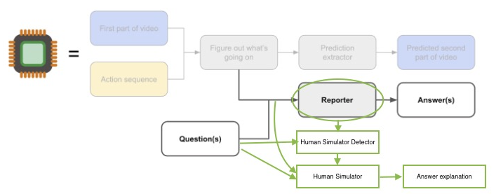
The overall strategy is to avoid training a “human simulator” reporter by regularizing its internal state to have mind-blindness. One could imagine training a “Human Simulator” that takes as input the “what’s going on” state, plus a question about what a human believes about the world, and is trained to maximize its accuracy at predicting the human’s answer explanation. Meanwhile, the Reporter is trained with dual objectives: in addition to (as before) answering questions about the world correctly, it should be penalized for containing internal state that is useful to the Human Simulator. To do this, an auxiliary “Human Simulator Detector” model is trained to predict the Human Simulator’s activations from the Reporter’s activations. The Reporter is trained adversarially to minimize the Human Simulator Detector’s accuracy. The reporter would be trained not merely to be bad at predicting the explanation — an evil reporter could pretend to be bad at predicting the explanation — but to not contain state that is predictive of “human simulator state”. This is something that the various defeated strategies are missing. A devious reporter can easily hide its full knowledge from its predicted answer, and may even choose weights to look like it does not contain a human simulator. But we argue that when operating on actual input data, a devious reporter will find it more challenging to run a simulation while pretending not to.

This strategy is depicted below:

More precise detail on strategy

The Reporter’s overall loss function to minimize takes the form:

reporter_loss

= reporter_prediction_loss – alpha * human_simulator_detector_loss.

How to find a strategy for choosing the hyperparameter alpha is an open question. But, if the Reporter can do just as well at reporting with and without containing a human simulator, then any positive alpha would be sufficient to choose not to contain a human simulator.

The Human Simulator assumes a form of data augmentation that allows us to train a model that knows how humans would interpret their observations of the world. In one embodiment depicted above, the human labeler will provide not only an answer, but an answer explanation. The Human Simulator would have the same inputs as the Reporter, but would predict this answer explanation rather than the answer. (Other possibilities can be envisioned. For example, the Human Simulator could be trained to predict both the answer and the answer explanation.)

The Human Simulator Detector takes in the Reporter’s internal state (activations) as input, and tries to predict the Human Simulator’s internal state (activations) as input (by training with MSE loss, for example). The Human Simulator Detector actually tries to minimize the

human_simulator_detector_loss

= simulator_state_mse_loss + gamma * ||human_simulator_detector.weights ||^2,

where the latter term can be replaced with some standard approach to minimizing its model complexity. If the Reporter contains a human simulator within itself identical to the Human Simulator, then the Human Simulator Detector will be able to predict the Human Simulator state by simply selecting such states (ie it will be the identity function for the portion of the Reporter that is its human simulator). Note that if the Reporter contains its human simulator activations in a permuted order from the Human Simulator, and if the Human Simulator Detector is a single-layer feedforward network, then it could simply learn a permutation matrix rather than the identity matrix.

On the other hand, if the Reporter does not contain a human simulator within itself, the Human Simulator Detector will either have high model complexity (simulating a human presumably requires a complex model — especially because it is not given “what’s going on” as input, but instead on the Reporter’s internal state, which contains less information according to the Data Processing Inequality), or it will have high simulator_state_mse_loss. Thus, the Reporter can be trained in an adversarial fashion, minimizing its own reporter_loss, while maximizing the human_simulator_detector_loss.

Counterexample

While I do not have a specific counterexample scenario that defeats this strategy, a “recipe” for a successful counterexample can be abstractly described. The scenario must be on in which it is easier for the Reporter to both learn its own simulator while also learning to disguise its simulator from the Human Simulator Detector, rather than learn to be an accurate reporter without learning a simulator. It would seem that standard regularization techniques applied to the Reporter would prefer the latter. So a counterexample would be one in which an accurate reporting would be difficult or impossible without human simulation.

Besides the possibility of counterexamples, this strategy could fail if one is unable to successfully train a Human Simulator Detector in the first place. To succeed we need to solve two problems that appear to be solvable yet practically challenging: training the Human Simulator, and training the Human Simulator Detector using the Human Simulator.

With regards to training the Human Simulator, the key challenge is obtaining labeled data that forces a model to not only reason about the video input, but also reason about how humans reason about the video input.

With regards to training the Human Simulator Detector, the model will have to map from a large input space to a large output space. However, because n_activations ~ sqrt(n_weights) in a feedforward neural network, the Human Simulator Detector would probably require roughly the same number of weights as the two other networks. We assume that the Human Simulator Detector can be trained to be permutation invariant with respect to Reporter activations. This is not as hard as it looks: as noted in the previous section, so long as the permutation of activations is the same across samples, then undoing this is a sparse linear transformation. If the permutation of activations varies among samples, then this would be harder.

This was originally published here: https://calvinmccarter.wordpress.com/2022/02/19/mind-blindness-strategy-for-eliciting-latent-knowledge/

#ML #futurism

The Newton Schulz iteration for matrix inversion

November 26, 2022

The Newton Schulz method is well-known, and the proof of convergence is widely available on the internet. Yet the derivation of the method itself is more obscure. Here it is:

We seek the zero of \( f: \mathbb{R}^2 \rightarrow \mathbb{R}^2\), defined as follows: \( f(X) = X^{-1} – A\).

The derivative of \(f\) at \(X\), applied to matrix \(B\), operates on \(B\) as follows: \[ \begin{array}{l} f'(X)[B] = -X^{-1} B X^{-1}. \end{array} \]

We can then prove that \( f'^{-1} \) at \( X \), applied to matrix \( B \), operates on \( B \) as follows: \( \begin{array}{l} f'^{-1}(X)[B] = -X B X \end{array} \).

To see this, notice that \[ \begin{array}{l} B \\ = f'^{-1}(X)\Big[f'(X)[B]\Big] \\ = -X \Big[-X^{-1} B X^{-1}\Big] X \\ = B. \end{array} \]

The Newton method for root finding has at each iterate: \[ \begin{array}{l} X_{t+1} \\ = X_t – f'^{-1}(X_t)\Big[f(X_t)\Big]\\ = X_t – f'^{-1}(X_t)\Big[X^{-1} – A\Big] \\ = X_t – X_t[X^{-1}_t-A] X_t \\ = X_t – [-X_t + X_t A X_t]\\ = 2 X_t – X_t A X_t \end{array} \].

This was originally published here: https://calvinmccarter.wordpress.com/2021/11/18/the-newton-schulz-iteration-for-matrix-inversion/

#ML

Preprocessing and cross-validation

November 26, 2022

From http://www.eigenvector.com/faq/index.php?id=153:

In general, preprocessing should be done inside of cross-validation routine. If you preprocess outside of the cross-validation algorithm (before calling crossval), you will bias the cross-validation results and likely overfit your model. The reason for this is that preprocessing will be based on the ENTIRE set of data but the cross-validation’s validity REQUIRES that the preprocessing be based ONLY on specific subsets of data. Why? Read on:

Cross-validation splits your data up into “n” subsets (lets say 3 for simplicity). Let say you have 12 samples and you’re only doing mean centering as your preprocessing (again, for simplicity). Cross-validation is going to take your 12 samples and split it into 3 groups (4 samples in each group).

In each cycle of the cross-validation, the algorithm leaves out one of those 3 groups (=4 samples=”validation set”) and does both preprocessing and model building from the remaining 8 samples (=”calibration set”). Recall that the preprocessing step here is to calculate the mean of the data and subtract it. Then it applies the preprocessing and model to the 4-sample validation set and looks at the error (and repeats this for each of the 3 sets). Here, applying the preprocessing is to take the mean calculated from the 8 samples and subtract it from the other 4 samples.

That last part is the key to why preprocessing BEFORE crossval is bad: when preprocessing is done INSIDE cross-validation (as it should be), the mean is calculated from the 8 samples that were left in and subtracted from them, and that same 8-sample mean is also subtracted from the 4 samples left out by cross-validation. However, if you mean-center BEFORE cross-validation, the mean is calculated from all 12 samples. The result is that, even though the rules of cross-validation say that the preprocessing (mean) and model are supposed to be calculated from only the calibration set, doing the preprocessing outside of cross-validation means all samples are influencing the preprocessing (mean).

With mean-centering, the effect isn’t as bad as it is for something like GLSW or OSC. These “multivariate filters” are far stronger preprocessing methods and operating on the entire data set can have a significant influence on the covariance (read: can have a much bigger effect of “cheating” and thus overfitting). The one time it doesn’t matter is when the preprocessing methods being done are “row-wise” only – that is, methods that operate on samples independently are not a problem. Methods like smoothing, derivatives, baselining, or normalization (other than MSC when based on the mean) operate on each sample independently and adding or removing samples from the data set has no effect on the others. In fact, to save time, our cross-validation routine recognizes when row-wise operations come first in the preprocessing sequence and does them outside of the cross-validation loop. The only time you can’t do these in advance is when another non-row-wise method happens prior to the row-wise method.

This was originally published here: https://calvinmccarter.wordpress.com/2015/08/19/preprocessing-and-cross-validation/

#ML